PID theory: Non-linear systems

More than any other section of this tutorial, you should treat this one as broad background rather than as instructions to be specifically applied. Even highly experienced control engineers tread VERY carefully when the word 'nonlinear' pops up. Amazingly, even with today's technology, there are no formal ways for dealing with nonlinear systems, and adding nonlinearity to a control system can cause very unpredictable behaviour. Basically, your approach should be to identify possible nonlinearities within your application - if it looks like there aren't any (careful, they're very good at hiding), breathe a sigh of relief and proceed. If there are, proceed anyway but consider getting some assistance if your application is critical. 

A non-linear system, in the context of closed loop control, is a system that contains elements whose output versus input graph is not a straight line. We are not talking here about the output versus time, but rather the final steady state output for a given input.

Consider our electric kettle. Suppose we connect it into a control system with a temperature sensor and an electronically controlled "dimmer" that produces an output voltage proportional to its input control voltage. Suppose the temperature sensor is linear (its output voltage is directly proportional to temperature). So we have a linear sensor and a linear element voltage versus control. Is the overall system therefore linear?

No, it's not. For a start, the heat generated by the element is proportional to power, not voltage. And for a resistive element power is voltage squared divided by resistance. So right there we have a square law not a linear law.

Secondly, remember we determined that our kettle needed 200W to hold the water temperature at 80Cº, (60ºC above an ambient of 20ºC). The kettle had a 2000W element. Hence, if we turn on full power the water will heat up by 10 times as much, i.e. 600ºC.

Hang on, hang on. Heat water up by 600ºC?

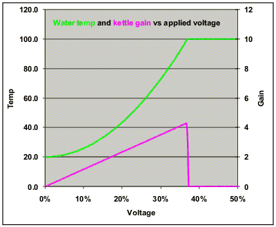
Water boils at 100ºC, so what happens if we pour 2000W continuously into the kettle? The water will boil, and at 100ºC it will get no hotter. Instead, the energy will all go into turning the water into steam, until it has all boiled away and we have a melted down kettle to explain to our spouse. Clearly, the temperature versus power graph flattens out at 100ºC, so temperature ceases to be proportional to power or to the square of voltage.

The graph shows the temperature in green, plotted against voltage expressed as a percentage of full voltage (120V or 240V, take your pick). The magenta plot is the "gain" of the kettle. Gain is the slope of the temperature versus voltage graph, and indicates the sensitivity to a voltage change. Gain varies with voltage. Below about 33% gain increases from zero to some maximum. It then drops sharply to 0.

The flattening of the green curve above 33% of voltage is called saturation or limiting (or boiling or melt-down in the case of our kettle).

All real systems saturate at some point. Nasty things can happen in a control system if you hit saturation. That means you need to carefully consider how and when your system may saturate, and make sure it will not go berserk if saturation is unavoidable at some time. If saturation is possible you will need to devise tests to force it into saturation to check its behaviour is acceptable.

Getting back to the non-linear gain (i.e. gain that varies across the operating range). Later you will learn that gain is one of the important parameters in a PID controller. The more gain, the more the system (controller + process) will tend to become unstable and oscillate. The less gain the less accurate the system will tend to be. You may therefore need to plot the gain of your process and then simulate and test at several points using the gain figures. You will also have to evaluate possible changes in gain due to external influences like temperature, supply voltage, friction or whatever.

The PIDassist program allows you some ability to simulate saturation but not other non-linearities. It also lets you set the gain of the simulated process.