PID theory: The control model
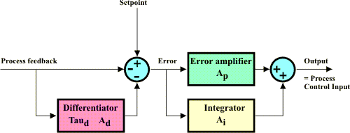
The actual PID controller is implemented in a SPLat (or any other digital controller) as a bunch of numerical calculations. There are several ways of performing the necessary calculations, depending on the exact "circuit configuration" your program is emulating. The program we use implements the configuration in the diagram.

In this diagram the circles represents summations or subtractions. Hence the left-hand circle calculates the setpoint minus the process feedback minus the derivative to produce an error signal. Arguably the derivative should be subtracted in the righthand "summer", but this way produces slightly simpler code and works just as well. The error is multiplied by Ap (proportional gain) in the green box and integrated in the yellow box, then the two are added together to produce the final controller output.
In the actual programs the derivative is calculated in slightly round-about way. Instead of calculating the difference between successive input samples (which would be the "natural" way of doing it), we put the input through one of the time constant calculations we have been studying earlier, to calculate a moving average, then subtract that from the direct input to get the derivative. For this reason the differentiator has an associated time constant Td ('Derivative time') as well as a gain setting Ad.
The integrator is implemented as an ongoing adding up of the error at each sample, times a scaling factor. The factor specifying integral is 'Integral time' - Ti - which is the time it takes for the output to ramp an amount equal to the prevailing controller error.
The error amplifier is just a multiplication by Ap.
The calculation, performed each sampling interval, goes like this:
- Let Kd = the factor required to get a time constant of Td
- Call the process feedback "Input"
Then:
- New_LPFin = Old_LPFin * (1-Kd) + Input * Kd (this is the moving average of the input, which in electronics parlance is the input lowpass filtered.
- Derivative = Input - New_LPFin
- Old_LPFin = New_LPFin (for next time)
- Error = SetPoint - Input - Derivative * Ad
- Integral = Integral + Error
- Output = Error * Ap + Integral
In practice, there is one other wrinkle. In our code we limit the range of integral values to the valid range of output values (the integrator is designed to "saturate"). This combats "integrator windup", where the integrator can build up excessive values if the process is slow to respond due to saturation elsewhere.
